Classification of Gravitational Waves from Black Hole-Neutron Star Mergers with Machine Learning

1. INTRODUCTION

Since the groundbreaking detection of gravitational waves (GWs) in September 2015 (Abbott et al. 2016) by the advanced Laser Interferometer Gravitational-Wave Observatory (LIGO) and the Virgo Collaboration (Abbott et al. 2009; Aasi et al. 2015; Acernese et al. 2015), the field of GW Astrophysics has entered a new epoch. In the initial observing runs, O1 and O2, a total of eleven GW signals from compact binary mergers were identified, encompassing ten binary black-hole (BBH) events and a singular, distinct binary neutron star (BNS) merger, GW170817 (Abbott et al. 2017b, 2019a, 2019b). The significance of GW170817 extended across scientific disciplines, marking the beginning of Multi-Messenger Astrophysics (MMA) by linking gravitational wave observations with electromagnetic (EM) radiation (Abbott et al. 2017c). This convergence unveiled a new horizon for understanding astrophysical processes using GWs, EM radiation, cosmic rays, and neutrinos, offering a comprehensive view of celestial sources (Vartanyan & Burrows, 2020; Yuan et al. 2020). As the third observing run (O3), which was divided into O3a and O3b, the number of gravitational wave events increased significantly, exceeding 70 new detections. Notably, this phase not only included an additional BNS merger (Abbott et al. 2020) but also witnessed, for the first time, the detection of two neutron star-black hole (NSBH) mergers (Abbott et al. 2021). The cumulative events, including those from O3, form the third Gravitational-Wave Transient Catalog (GWTC-3), incorporating over 90 distinct occurrences of compact object mergers (Abbott et al. 2023a, 2023b).

The start of the O4 observing run in May 2023 heralds an ambitious 20-month phase for LIGO, Virgo, and KAGRA collaborations. O4a, the initial period, concludes on January 16, 2024, marked by endeavors to address variable noise coupling. Following an 8-week break and an engineering run (ER16) in March 2024, O4b commences on March 27, 2024, marking a key phase for gravitational wave observations. LIGO’s Hanford and Livingston detectors sustain robust operation, exhibiting a BNS detection range of 140 to 170 Mpc. Meanwhile, Virgo is expected to achieve a BNS range over 45 Mpc due to recent commissioning efforts aimed at noise reduction and stability improvements. Plans for the subsequent O5 remain under revision by Virgo, with details expected to solidify by mid-2024. KAGRA’s reinitiated commissioning, scheduled to rejoin observations in spring 2024, anticipates a BNS range of around 10 Mpc (Abbott et al. 2017a; 2018; Cahillane & Mansell 2022).

However, the increasing detection rates of GW pose a computational challenge for current matched-filtering techniques (Antelis & Moreno 2019). These traditional methods, relying on pre-calculated waveform templates, become computationally intensive and need help with the expansive parameter space of unknown source characteristics (Canton et al. 2014). Moreover, their dependence on precise templates raises concerns about potential missed signals that deviate from expected theoretical patterns (Gabbard et al. 2018; Kang et al. 2022). Additionally, accounting for unique events with factors such as eccentricity, precession, and higher-order models makes it impractical to cover this range with millions of templates, especially in neutron star scenarios where prompt electromagnetic follow-ups are crucial (Kang et al. 2022).

Consequently, the pressing demand for more efficient detection and classification algorithms in astronomy, overcoming the limitations of conventional methods, has led to the emergence of Deep Learning (DL) methodologies. Recently, Qiu et al. (2023) demonstrated the success of DL in identifying coalescence GW events involving neutron stars, encompassing two BNS mergers and two NSBH mergers (Qiu et al. 2023). These advances in DL, along with the increasing prevalence of machine learning techniques are playing crucial roles in tasks such as exploring supernova GWs (Mitra et al. 2023), optimizing efficiency and accuracy in estimating the detectability of extreme-mass-ratio inspirals signals (Chapman-Bird et al. 2023; Yun et al. 2023), and gravitational wave data analysis (Gabbard et al. 2018; George & Huerta. 2018; Dreissigacker et al. 2019; Ormiston et al. 2020; Wang et al. 2020; Zhanabaev & Ussipov 2023), reflecting their growing significance in advancing astronomical research. The utilization of Convolutional Neural Network (CNN) algorithms has demonstrated remarkable potential in detecting simulated signals from BBH collisions amidst Gaussian noise, rivaling or surpassing the performance of conventional matched-filtering techniques (Qiu et al. 2023). This marked a turning point, prompting numerous research cohorts to embrace DL algorithms for detecting GW BBH events in simulated and real LIGO data.

Considering the computational challenges faced by current matched-filtering techniques in GW detection, as mentioned earlier, our research introduces conditional information as a novel feature for signal characterization. Entropy, a ubiquitous tool in signal processing, offers a unique perspective for characterizing signal attributes, effectively addressing the limitations inherent in traditional methods. Its application is widespread across various disciplines, such as radar signal processing for source attribution and signal classification (Nalband et al. 2018; Zhang et al. 2023), and in the medical field for disease diagnosis through electroencephalograms (EEGs) or electrocardiograms (ECGs) analysis (Chawale et al. 2022). By incorporating entropy analysis into our GW detection and classification methodology, we aim to enhance the versatility and effectiveness of GW detection algorithms. This approach represents a significant departure from the prevailing deep learning methods. It could potentially offer a more efficient solution to the challenges of large parameter spaces and the need for prompt identification in scenarios involving neutron stars.

Considering the computational challenges faced by current matched-filtering techniques in GW detection, this research introduces conditional information as a novel feature for signal characterization. Conditional information estimation involves analyzing two discrete time series: the received GW signal and signal interference. By leveraging mutual information, which quantifies the nonlinear relationship between these signals, the methodology addresses limitations inherent in traditional methods. This approach represents a significant shift from conventional deep learning methods, offering a potentially more efficient solution to the challenges of large parameter spaces and prompt identification, especially in scenarios involving neutron stars.

The rest of the paper is structured as follows. In section 2, we describe our methods to construct a dataset, calculate conditional information, and train CNNs. In section 3, we present and discuss the results. In section 4, we make conclusions.

2. DATA AND METHODS

2.1 Data Preparation

For the simulation of GW signals for Compact Binary Coalescences (CBC), we utilized the LIGO Algorithm Library Suite (LALSuite; LIGO Scientific Collaboration 2018). This suite provided us with the tools to generate waveforms for BBH, BNS, and NSBH systems. The specific time-domain waveform approximants used were SEOBNRv4 for BBH (Bohé et al. 2017), which models the inspiral, merger, and ringdown components of the signal, TaylorF2 for BNS (Messina et al. 2019) and IMRPhenomNSBH for NSBH (Matas et al. 2020). Our approach is adapted by the widely used methodology of Gebhard et al. (2019), which we integrated for our own needs. The generated signals are illustrated in Fig. 1.

Fig. 1. Sample of simulated gravitational waves (GWs) projected onto the Hanford (H), Livingston (L), Virgo (V) detectors.

Download Original Figure

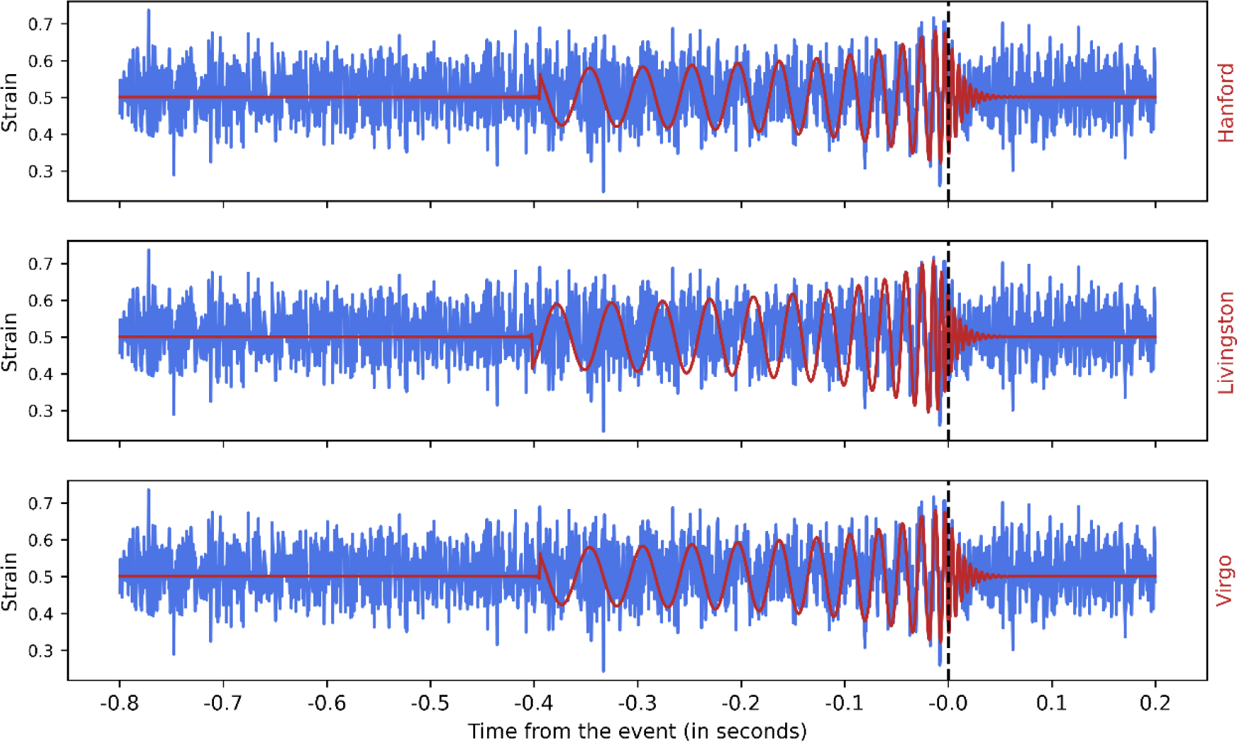
In creating BBH waveforms, we uniformly sampled component masses between 2 and 95 M_☉ with a maximum mass ratio (m₁/m₂) of 10. For BNS waveforms, the component masses were uniformly sampled between 1 and 2 M_☉. For NSBH waveforms, neutron star component masses were uniformly chosen between 1 and 2 M_☉, while black hole masses were sampled between 2 and 35 M_☉. We randomly sampled values for the z-components of their spins, right ascension, declination, polarization, inclination, and coalescence phase angle. These parameters collectively specify the location and orientation of the source in the sky, as well as the injection signal-to-noise ratio (SNR).

Waveforms are sampled at a frequency of 4,096 Hz over 4 seconds. This duration was chosen by the authors (Qiu et al. 2023) as it has proven effective in achieving robust discrimination between different classes of CBC. Moreover, this timeframe is sufficient for accurately recovering real GW signals corresponding to all CBC configurations. Opting for these shorter templates significantly reduces memory requirements during our neural network training, a crucial factor in managing computational resources effectively.

To simulate realistic GW signals, we inject GW signals into Gaussian noise using the PyCBC library, which utilizes the power spectral density (PSD) model specific to the advanced LIGO detectors (Usman et al. 2016; Biwer et al. 2019). Gaussian noise is generated to match the expected background noise characteristics for the detector. The GW signals are then projected on the detectors and resized before being injected into the Gaussian noise with a specific SNR. Real data from the detectors as well as simulated signals undergo a whitening process to enhance the signal visibility against background noise. Whitening is performed using PSD computed directly from the raw gravitational wave strain data via Welch’s method (Welch 1967). This critical step ensures that the noise contribution at each frequency is rescaled to have equal power, thereby making the signal more distinct. Whitening is a linear operation; thus, applying it separately to both real data and simulated signals is effectively equivalent to whitening the combined data, as noted by Gabbard et al. (2018).

To further refine our training process and make it robust against moderate time translations in the signal, we randomly position the peak of each waveform within the template, specifically between 3.7 and 3.9 seconds. This randomness in peak positioning enhances the model’s ability to handle moderate time translations in the signal during training (Qiu et al. 2023). Additionally, we adjust the amplitude of each injected waveform to achieve a specific SNR. The SNR is defined as follows (Gabbard et al. 2018):

$${\rho }_{opt}^2=4{\displaystyle \underset{f_{\min }}{\overset{\infty }{\int }}\frac{\left|h^{~}\left(f\right)\right|}{s_n\left(f\right)}df}$$

(1)

where h˜ is the frequency domain representation of the GW strain, S_n(f) is the single-sided detector noise PSD, and f_min is the frequency of the GW signal at the start of the sample time series. From an astrophysical perspective, rescaling the waveform is equivalent to varying the source distance from the detector.

We generate 480,000 templates for training, 16,000 templates for validation, and 1,600,000 templates for testing, all disjointing. SNR was uniformly sampled in the range between 0 and 20.

2.3 Convolutional Neural Network

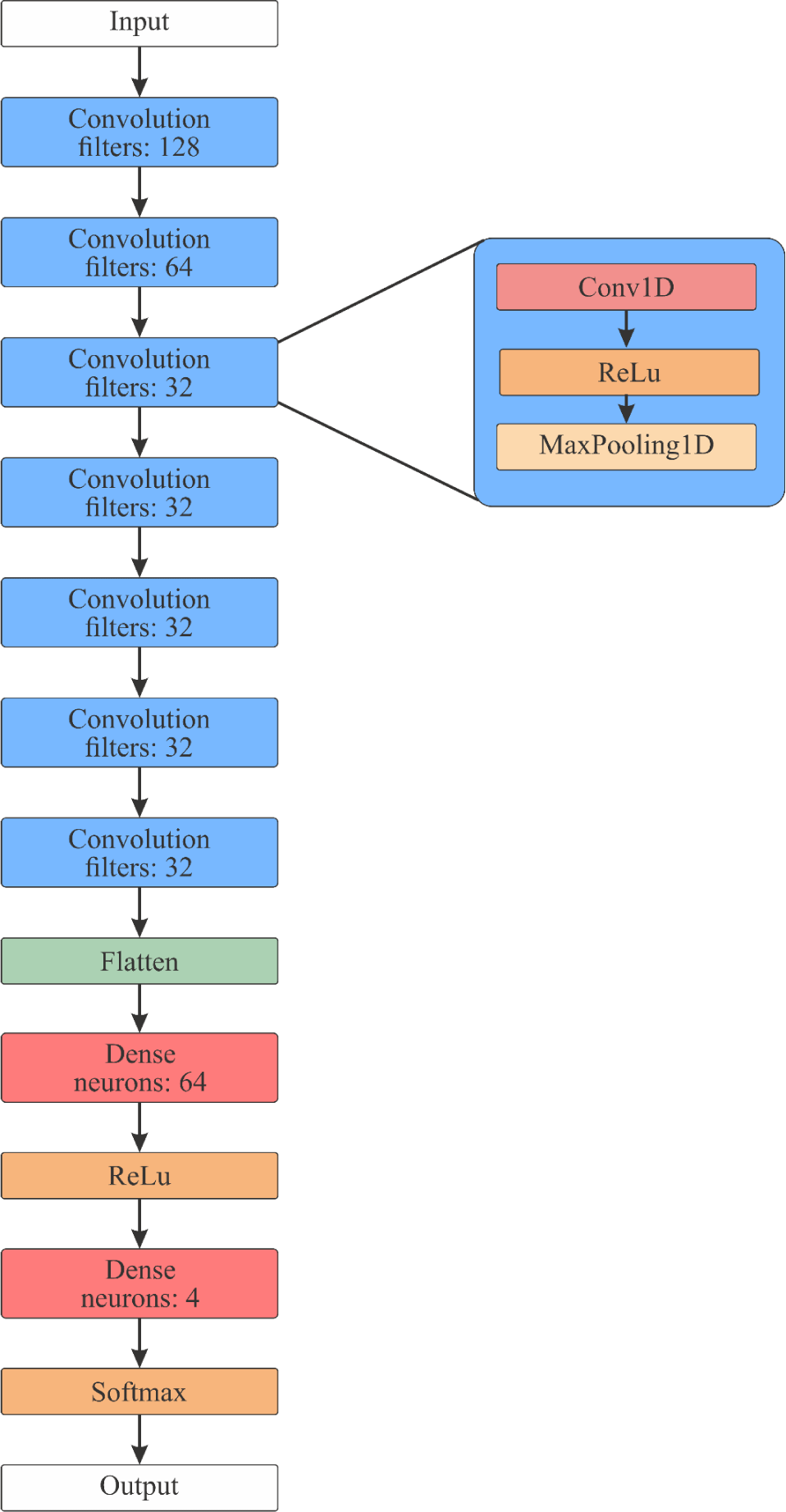
Fig. 2 shows CNN processing the input time series, where convolutional filters slide over the data to extract local patterns and temporal dependencies. This method helps the network learn key data characteristics. Pooling layers reduce dimensionality, and the final softmax layer outputs probabilities for categories like BBH, BNS, NSBH, or Noise, ensuring accurate classification.

Fig. 2. Using Conditional entropy as a feature to classify gravitational wave (GW) signals. The red arrow illustrates the movement of the convolutional filters as they traverse the input time-series vector. The final layer outputs the probability that the input time series is classified into one of the categories: binary black-hole (BBH), binary neutron star (BNS), neutron star-black hole (NSBH) or Noise.

Download Original Figure

Our CNN architecture comprises 7 convolutional blocks followed by 2 Dense layers, concluding with a softmax activation function at the output. Each convolutional block features a 1D convolution layer with a ReLU activation function and a 1D Max Pooling layer. The parameters for the Conv1D and MaxPooling1D layers are set as follows: kernel size of 3 for Conv1D, pool size of 2 for MaxPooling, and same-padding for both layers. The convolutional layers are configured with 128, 64, 32, 32, 32, 32, and 32 filters, respectively, while the Dense layers consist of 64 neurons in the hidden layer and 4 neurons in the output layer. The model has a total of 175,140 parameters. The CNN model was implemented and trained using TensorFlow 2.1, with the Adam optimizer, a learning rate of 0.001, and a batch size of 256. We utilized categorical cross-entropy as the loss function and incorporated EarlyStopping regularization, monitoring validation accuracy with a patience of 10 epochs. The training was performed on an NVIDIA GeForce RTX 3080 GPU with 10 GB of video memory. The architecture is illustrated in Fig. 3.

Fig. 3. A schematic diagram of neural network architecture illustrates that all 1D convolution layers within a given convolutional block have various numbers of filters. The total number of parameters in the model is 175,140.

Download Original Figure

3. RESULTS AND DISCUSSION

We evaluate the performance of our model using a testing dataset consisting of GW events described in subsection 2.1. This evaluation includes assessing the effectiveness of our approach within the impact of SNR, accuracy of CNN within training progress and comparing the trained DL model’s performance before and after with utilizing our approach. Finally, the model’s performance is tested on real GW events from the GWTC-3 catalog.

Fig. 4(a) depicts the conditional information and entropy calculations for three types of gravitational wave signals: BBH, BNS, and NSBH. These values are calculated using Eqs. (4) and (5), with the peak interval of the time series data used for the calculations. We then applied the Monte Carlo method to average the conditional information and entropy across all simulated data. The results show distinct levels of conditional information and entropy for each signal type, indicating its potential as a feature for classification.

Fig. 4. Impact of varying signal-to-noise ratio (SNR) and window size. (a) Conditional information (dashed) and conditional entropy (solid) of different signals with increasing SNR. (b) Conditional information (dashed) and conditional entropy (solid) of different signals with different window sizes.

Download Original Figure

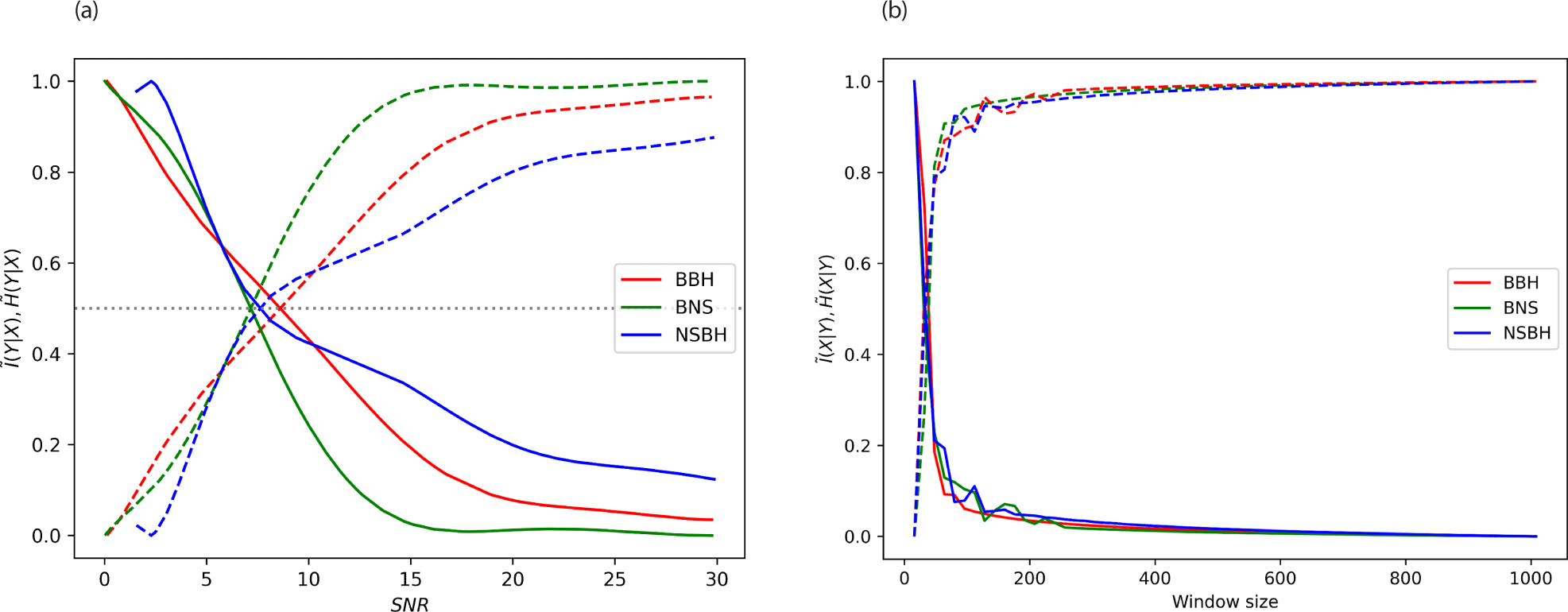
The three curves show that as the SNR increases, the probability of detecting BBH and NSBH increases rapidly and then levels off, indicating that higher SNR values do not significantly increase the detection probability. For BNS events, the probability increases more gradually and continues to increase as SNR grows.

At lower SNR values, BNS events have a higher detection probability than BBH and NSBH, but as the SNR increases, the probability for BBH and NSBH surpasses that of BNS. This could imply that BBH and NSBH events produce stronger signals at higher SNRs, making them easier to detect compared to BNS events.

Fig. 4(b) shows the variation of conditional information and entropy with different window sizes, using an SNR of 30. The figure demonstrates that the feature remains stable within a particular window size.

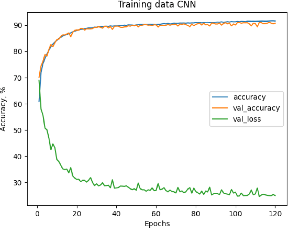
The performance of our CNN model was evaluated based on its ability to correctly classify simulated GW signals into their respective categories: BBH, BNS, and NSBH. Fig. 5 shows training progress of a CNN over a certain number of epochs, which are iterations over the entire data set. Both the accuracy and validation accuracy are converging to a high percentage, and the validation loss is decreasing, which indicates that the model is learning effectively without overfitting, as there is not a significant gap between training and validation accuracy.

Fig. 5. Training process of Convolutional Neural Network (CNN) model.

Download Original Figure

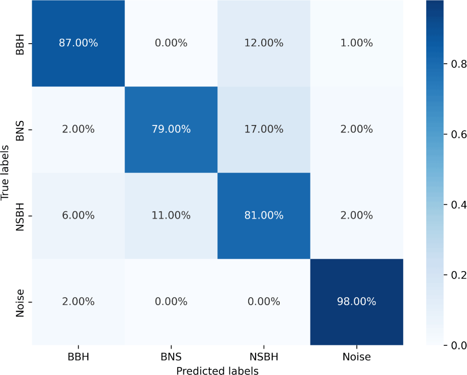
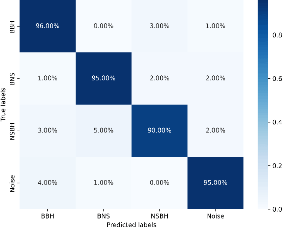
Two confusion matrices are included to illustrate the impact of incorporating conditional information into CNN training. Fig. 6 shows the confusion matrix before integrating conditional information, while Fig. 7 presents the results after its inclusion. The comparison reveals significant gains in classification accuracy and model performance, showing that conditional information effectively refines the network’s ability to differentiate between gravitational wave signal types. After integrating conditional information, the model shows the following performance metrics:

Fig. 6. The confusion matrix for standard time series training.

Download Original Figure

Fig. 7. The confusion matrix utilized conditional entropy as a feature for training.

Download Original Figure

An analysis of real gravitational wave events from GWTC-3 is included to assess the effectiveness of the methodology. Table 1 presents the classification results for these events, detailing the gravitational wave signals identified by the model. The table includes the event name, masses, detected SNR, and the type of CBC.

4. CONCLUSION

Our research has successfully demonstrated the viability of employing machine learning techniques, particularly CNNs and conditional information estimation, for the classification of gravitational wave signals from BH-NS mergers.

We introduced an innovative methodology that combines conditional information as a feature in signal processing with the power of deep learning for gravitational wave detection. This approach not only addresses the limitations of traditional matched-filtering techniques but also enhances the detection and classification accuracy of GW signals.

We constructed a comprehensive dataset of simulated gravitational wave signals using the LALSuite. This dataset, including waveforms for BBH, BNS, and NSBH systems, was pivotal in training and validating our CNN model, ensuring its robustness and accuracy in real-world scenarios.

The CNN model exhibited exceptional performance, achieving high accuracy rates in classifying simulated GW signals into their respective categories. This level of accuracy is particularly significant considering the complexities involved in distinguishing between different types of gravitational wave signals.

Our methodology’s applicability to real gravitational wave data was validated by testing the model on real GW data from the GWTC-3 catalog, where it achieved notable accuracy. This underscores the potential of our approach in contributing to ongoing and future gravitational wave observational campaigns.

The promising results of our study pave the way for further research and development in the field. With the anticipated improvements in gravitational wave detectors and the continuous evolution of machine learning algorithms, the scope for more refined and advanced detection methods is vast. Our research contributes a foundational step towards this progress.