1. INTRODUCTION
Variable stars are defined as stars that change in brightness, with periods from a few seconds to hundreds of years. They are classified as pulsating variable stars, eruptive or cataclysmic variable stars, and eclipsing variable stars, depending on the factors and physical characteristics that cause the brightness change (Petit 1987). For pulsating variable stars, the brightness changes because of the change in surface temperature that occurs as the stars repeatedly contract and expand at regular intervals. The nature of this contraction and expansion depends on the equilibrium relationship between gravity and radiation pressure. RR Lyr, Cepheid, and Mira type stars are representative examples. For eruptive or cataclysmic variable stars, sudden changes in brightness originate from abrupt explosions caused by stellar flare emission, stellar atmospheric matter emission, and mass influx from accompanying stars. Flare stars, novae, and supernovae belong to this classification. For eclipsing variable stars, periodic changes in apparent brightness can be observed in cases where the orbital planes of two stars almost coincide with the line of sight. Representative examples are Algol, β Lyr, and W UMa type stars. These variable stars are continuously researched because they provide information on the physical characteristics and evolution of stars, and such information is very useful for revealing basic knowledge of the universe.
With the development of technologies used for exploring variable stars, various projects have been undertaken to date. LOTIS (Park et al. 1997) and ROTSE-III (Akerlof et al. 2003) were undertaken to observe gamma-ray explosion objects; OGLE (Udalski et al. 1992), MACHO (Alcock et al. 1993), and EROS (Aubourg et al. 1995) were established to observe gravitational microlensing; SPACEWATCH (Scotti et al. 1992), NEAT (Pravdo et al. 1999), and LINEAR (Stokes et al. 2000) aimed to explore and monitor near-Earth objects (NEOs); and ASAS (Pojmanski 1997), FSVS (Groot et al. 2003), and QUEST (Vivas et al. 2001) have searched for light variations throughout the whole sky. Byeon (2008) noted that data from such big monitoring programs, including SDSS (York et al. 2000), can be used to detect light variations for finding variable stars.
From its opening in 2008, the Chungbuk National University Observatory in Jincheon (hereafter, CBNUO) began performing time-series observations of variable stars using a 1-m RC-type reflecting telescope and 2K CCD. Currently, CBNUO is actively conducting time-series observations of variable stars using a 0.6-m wide-field telescope and 4K CCD, installed in 2010. Although several areas have been observed for more than 20 days among the observational data, no study has previously been undertaken on stars in the observation field except for the analysis of the target stars themselves. However, such an effort will improve the effectiveness of the data. Therefore, a period analysis algorithm was developed using World Coordinate System (WCS) Tools and the software of Shin & Byun (2004) to detect new variable star candidates in the observation areas. The developed algorithm was applied to the data of DO Dra (67 days), TT Ari (48 days), RXSJ1803 (39 days), and MU Cam (30 days), which were observed using CCDs with different fields of view, to examine the possibility of detecting new variable stars and the applicability of the algorithm to different fields of view.
2. OBSERVATIONAL DATA
The observational data used in this study were obtained using a 0.6-m wide-field telescope, ST-8 CCD, STX- 16803 CCD, and R filter at the CBNUO. The 0.6-m widefield telescope was constructed by the Korea Institute of Machinery and Materials as a part of the observation system for whole-sky exploration. It has a fork-type equatorial mount driven by sliding friction, and the driving speed goes up to 30 degrees per second. The optical system consists of a 0.6-m prime-focus-type primary mirror with f/2.92, fabricated by AstroOptik in Germany, and three correction lenses (Yoon et al. 2006). The detectors used were the ST-8 CCD from SBIG and the STX-16803 CCD. The field of view of the ST-8 CCD was 27′ × 18′, whereas that of the STX-16803 CCD, which was substituted for the ST-8 CCD on November 28, 2012, was 72′ × 72′. The field of view increased by a factor of 12 compared with that when the ST-8 CCD was used, as shown in Fig. 1, and the number of stars detected in the observation area increased by a factor of five.
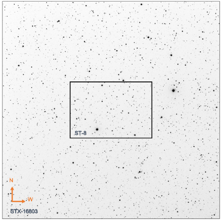
Sky areas for applying the developed period analysis algorithm to detect variable star candidates were selected when our time-series observation data of magnetic cataclysmic variable stars satisfied two conditions. The first condition was that the period of observation must be long; the number of observed days must be 20 or higher. The period of brightness change is not only an important physical parameter for a variable star but also an absolute requirement to retrieve the profile of the light curve (Shin & Byun 2004). Periods of variable stars range from short periods of less than one day to long periods of greater than 1,000 days. To detect variable star candidates with such periods, areas with long periods of observation and many days of observation are useful for the period analysis. In particular, these long periods are beneficial in detecting long-period variable stars that are usually difficult to observe.
The second condition is that both the 2K CCD and 4K CCD must have been used to observe these areas. For the CBNUO, replacing the 2K CCD with the 4K CCD expanded the field of view, and thus increased the number of stars available for observation. The developed algorithm must be applicable to areas covered by the previous observational data as well as stars added to the current observational data without additional software modification, irrespective of the change in field of view due to the CCD replacement. Observational data of DO Dra, TT Ari, RXSJ1803, and MU Cam were selected for the period analysis and variable star search, as shown in Table 1.

|
3. DATA ANALYSIS AND THE ALGORITHM FOR SEARCHING FOR VARIABLE STARS
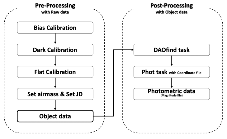
Data reduction was carried out using the image reduction & analysis facility (IRAF) package, which is provided by the National Optical Astronomy Observatory (NOAO) and is applied in general data reduction of astronomical observations. After pre-processing including bias calibration, dark calibration, and flat calibration, photometric data can be obtained based on the aperture photometry. Fig. 2 illustrates the process of obtaining the instrumental magnitudes of all the stars observed as point sources in the photometric observations.
One of the main purposes of this study was to develop an algorithm for finding variable stars present in the observed images around magnetic cataclysmic variable stars. The data were originally obtained to monitor the long-term periodic changes in the magnetic cataclysmic variable stars. The first step for this purpose was to find stars present in the observed images using the “DAOfind” task of the IRAF package. This task assigned an ID number to each point source in the observed images, whenever this source could be regarded as a star. Because the number of point sources is different in each observed image, a different ID number can be given to the same star. In the cases where the image is slightly rotated, no ID number can be given to the star. One reference file was made for each target field to include as many stars as possible. We calculated the movement value of each observed star and assigned it the ID number in the reference file. Making a suitable reference file was not simple; difficulties arose when some stars were not identified in the reference file because of bad weather, when the field of view was changed, and when the observed image was slightly rotated because of attachment and detachment of the CCD. In particular, the rotation of the observed image associated with the replacement of the CCD may cause a situation in which the center of rotation does not coincide with that of the observed image because of errors at the time of manufacturing. To address this problem, WCSTools was used in this study. WCSTools uses the USNO-B1.0 catalog (Monet et al. 2003). The process to correct the areas rotated by a few degrees, assign the same IDs to the stars included in images even if the image size or the number of recognized stars changed, and easily identify the characteristics of the stars using the assigned catalog IDs is described as follows.
A WCS astronomical image connects each pixel in an image to a specific direction of the sky. Therefore, stars in images can be found using the already known sky coordinates and the coordinates of stars found in images can be obtained (Mink 1997).
The currently available USNO-B catalog version 1.0 includes information on the five observation areas in the northern sky, four observation areas in the southern sky, colors, and epochs. This catalog contains an integrated list of the current positions, proper motions, magnitudes of various colors, classifications as stars or galaxies, and various measurements of 1,042,618,261 celestial bodies. Moreover, it has a position accuracy of 0s.2, and a photometric accuracy of magnitude 0.3 for J2000 coordinates for all sky areas, with perfect data up to magnitude 21 in V-filter (Monet et al. 2003).
Before the right ascension (RA) and declination (DEC) of the observed image could be calculated using imWCS from WCSTools, input of CDELT1, CDELT2, CTYPE1, and CTYPE2 keywords into the header information was first needed. CDELT1 and CDELT2 are values of WCS in degrees (°), which vary in each axis per unit pixel and have different values according to the pixel scale of the CCD. Table 2 provides a detailed description of the keywords. Among the keywords, the CDELT values also vary with the pixel scale. Therefore, these keywords were applied to the data from the CBNUO after proper modification. WCSTools can also easily be used with other observatories by simply adding the plate scale.
Because our data were observed to monitor magnetic cataclysmic variables, the target star was located at the center of each image. The RA (J2000) and DEC (J2000) of this star were set as the center coordinates, and a photometric program was used to find all stars in the image and sort their instrumental magnitudes. Bertin (1996) developed SExtractor program in WCSTools, which has high computational speed and is easy to use, therefore it is currently one of the most widely used photometry software programs. However, Roh (2002) insisted that SExtractor cannot be used for very accurate photometry results because it was developed only for moderate accuracy with proper calculation speed. Thus, instead of using the SExtractor software, we used “IRAF phot” to obtain photometric results for our data and to sort the instrumental magnitudes of stars in the image field. After photometry and sorting, the “ucatextractor” task was carried out to create a star list by comparing the resulting star list with the USNO-B1.0 catalog. Fig. 3 shows the process of obtaining WCS information. In this process, the results of ucatextractor are compared with the catalog, using the uidmatch software after the completion of imWCS, and the information of the identified stars as well as USNO-B1.0 IDs (hereafter IDs) are then written in cat files.
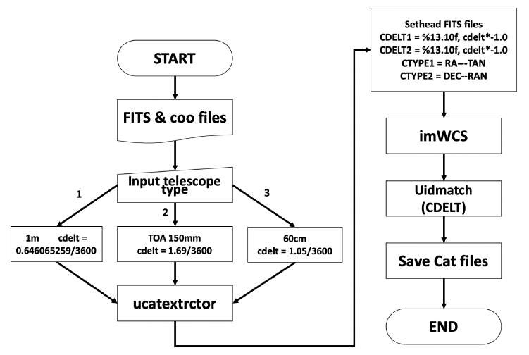
Each result of WCSTools was written in a cat file, where all information of identified stars from each image was recorded. All cat files were sorted in descending order of size. The biggest cat file would be that with the largest number of stars identified in the corresponding image. This file was selected as a reference file. Text files with each ID number were created, and the heliocentric Julian date (HJD), instrumental magnitude, and error of the instrumental magnitude were written in each text file of the corresponding ID. The number of text files was thus the same as the number of stars identified in the reference image. The file with the largest capacity was selected first to minimize the repetition of the ID classification process by selecting many stars from the beginning. The IDs stored in the reference file were compared with those recorded in the remaining cat files. If the IDs matched, the corresponding text files were recorded. Otherwise, the IDs were compared with those from other cat files. As this process was repeated, the capacity of the cat files was reduced. The process was repeated until the capacity of all cat files became zero, and the ID classification task was then terminated. All identified stars were thus assigned to USNO-B1.0 IDs, and their photometric information was stored in the text file with the corresponding ID number. The light curve of each star could then be constructed and used for period analysis. This process is shown in Fig. 4.
The observed images used in this study were from areas with stars fainter than magnitude 15. Therefore, it was exceedingly difficult to perform the standardization process. The comparison star used originally for the magnetic cataclysmic variable was also used as the comparison star in this study. The Δmag, which represents the difference between the magnitude of the comparison star and that of each star with an ID in the main image, was calculated and used for the period analysis. Period analysis was carried out according to the method suggested by Shin & Byun (2004).
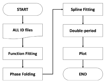
For the function fitting and phase folding, the periodic orthogonal polynomial method of Schwarzenberg-Czemy (1996) and the phase dispersion minimization method of Schwarzenberg-Czemy (1997) were used to find the starting value of the possible period. The reason these two methods were used was to examine the reliability of each method and determine the period more accurately. However, it should be noted that the incorrect period will be determined when the range of input frequencies is too small or too large. Thus, care must be taken in this step.
Shin & Byun (2004) also found that the function fitting and phase folding methods, which have been widely used for period analysis, are not always the best solutions because they often produce contradictory results. The most suitable periods were determined by performing spline fitting based on the cubic spline method of Akerlof et al. (1994), which finds the most suitable period for which kai2 is the minimum, using the sum of the cubic splines for the least squares method. However, the efficiency of this method is lower than that of the two above-mentioned methods, and this method sometimes presents results in a local optimum instead of the global minimum. Therefore, we carried out function fitting and phase folding first to reduce the possible period range, and then determined the most suitable periods using this method. For stars whose periodicity was obtained by this process, the light curve can be drawn using the calculated phase. For stars that showed the typical forms of eclipsing and pulsating variable stars, the periods with the best-fitting forms were selected based on visual inspection, and were determined as the periods of the stars. Stars without special patterns were excluded. Fig. 5 shows the period analysis process, including function fitting, phase folding, spline fitting, and plotting.
4. RESULTS AND CONCLUSIONS
CBNUO data for the monitoring and observation of magnetic cataclysmic variable stars were reanalyzed. As a result, 13 variable star candidates were found in the areas of DO Dra, TT Ari, RXSJ1803, and MU Cam, as shown in Fig. 6.
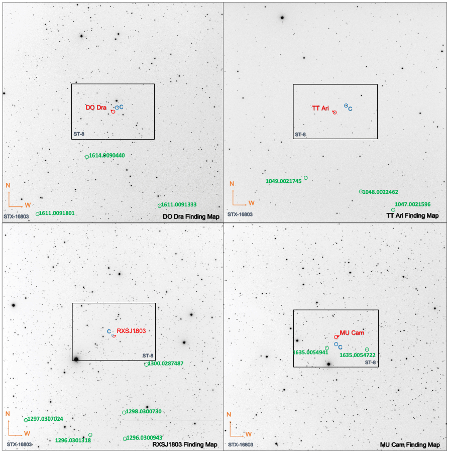
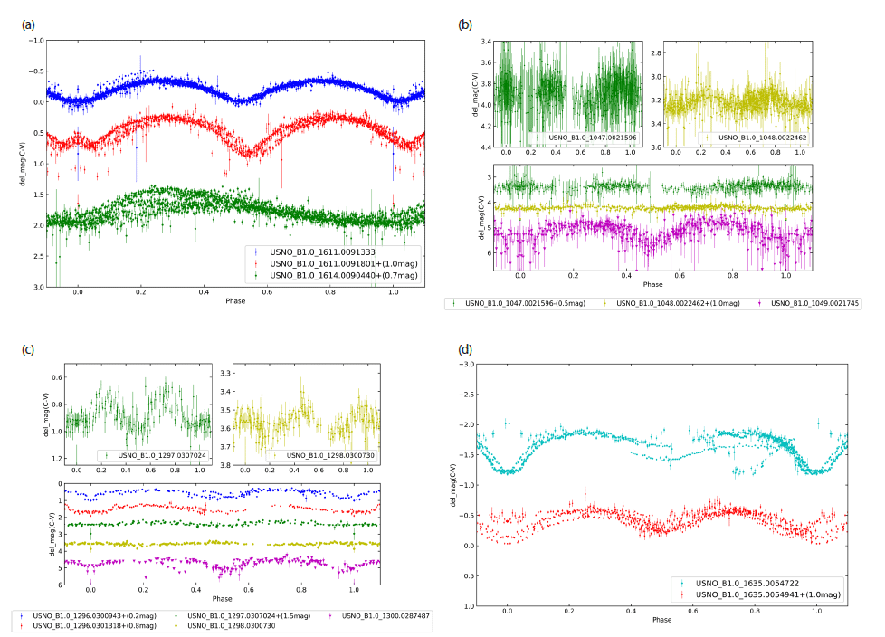
The sidereal period of DO Dra, a magnetic cataclysmic variable star, was 0.16537398 d (Haswell et al. 1997), and its rotation period was 529.31 s. Based on the CBNUO data corresponding to 67 days of observations from May 11, 2011 to April 22, 2014, variable stars were found using the developed algorithm. Two variable stars were confirmed, and one candidate was found by the period analysis. USNO-B1.0 1611.0091333 was detected as a variable star with a period of 0.434913260 d. Virnina (2011) proposed this star as a W UMa-type variable star with a period of 0.43911 ± 0.000009 d. USNO-B1.0 1611.0091801 was detected as a variable star with a period of 0.376817300 d. Virnina (2011) proposed this star as a W UMa-type variable star with a period of 0.376832 ± 0.000006 d. USNO-B1.0 1614.0090440 was detected as a variable star candidate with an expected period of 0.35390634 d. This star is considered to be a newly found variable star because no photometric analysis data could yet be found for it.
TT Ari is one of the brightest cataclysmic variable stars with a sidereal period of 0.13755 d (Belova et al. 2013). Three variable stars were detected using the data corresponding to 48 days of observations from October 6, 2009 to January 23, 2014. USNO-B1.0 1047.0021596 was detected as a variable star with a period of 0.569296440 d. Virnina (2010) proposed this star as a W UMa-type variable star with a period of 0.569332 ± 0.00015 d. However, the W UMa profile was not confirmed in this study. USNO-B1.0 1048.0022462 was detected as a variable star with a period of 0.36199440 d, and Virnina (2010) proposed a period of 0.331849 ± 0.000011 d. USNO-B1.0 1049.0021745 was detected as a variable star with a period of 0.223453680 d. Virnina (2010) proposed this star as a W UMa-type variable star with a period of 0.223445 ± 0.000001 d.
RXSJ1803, which was first named as an intermediate polar-type magnetic cataclysmic variable star by Gansicke (2005), has a sidereal period of 0.111257 d and a rotation period of 0.017599 d in a high state. Period analysis was attempted using the monitoring data corresponding to 39 days of observations from May 16, 2011 to April 8, 2014. Consequently, one variable star and four variable star candidates were found. USNO-B1.0 1296.0300943 (0.377485380 d), USNO-B1.0 1296.0301318 (0.590534620 d), USNO-B1.0 1297.0307024 (0.149456680 d), and USNO-B1.0 1298.0300730 (0.594111040 d) are considered newly found variable stars because no photometric analysis data have been reported for them. USNO-B1.0 1300.0287487 was detected as a variable star with a period of 0.334609320 d. Andronov et al. (2012) proposed this star as an Algol-type variable star with a period of 0.3348837 ± 0.0000002 d.
MU Cam was first named by Kazarovets et al. (2006). It is a magnetic cataclysmic variable star with a sidereal period of 0.19661 d and a rotation period of 0.01374127 d. Two variable stars were found using MU Cam observational data comprising 30 days of observations from December 12, 2011 to March 30, 2014. USNO-B1.0 1635.0054722 was detected as a variable star with a period of 1.151816860 d. Khruslov (2006) proposed this star as a β Lyr-type variable star with a period of 1.1514 d, and it was named V440 Cam by Kazarovets et al. (2011). USNO-B1.0 1635.0054941 was detected as a variable star with a period of 0.442890700 d. Khruslov (2006) proposed this star as a W UMa-type variable star, and Breus et al. (2010) determined the period to be 0.44264511 d. This star was named V442 Cam by Kazarovets et al. (2011).
The light curves of the 13 variable stars detected in this study are shown in Fig. 7, and their positions and periods are summarized in Table 3.
This study suggests the possibility of recycling CCD photometric observational data for research. Unlike photoelectric photometric observations, observations of CCD photometry contain information on other stars around the target star as well as the target star itself. After photometric study of the target star, these photometric images had not been used for further purposes. Since its opening in 2008, the CBNUO has also performed time-series observations of variable stars using a 1-m RC-type telescope and a 60-cm widefield telescope. In this study, an algorithm was developed to recycle time-series observation images and detect variable star candidates present in the images of the CBNUO. The above results were obtained by applying the developed algorithm to the observational data of the areas of DO Dra, TT Ari, RXSJ1803, and MU Cam with more than 20 days of observations among the time-series observational data of the CBNUO for the monitoring of magnetic cataclysmic variable stars.
If the developed algorithm is applied to time-series observation images, more variable stars can be found, and their physical characteristics can be identified. Moreover, we have also developed an algorithm for finding asteroids (Kim 2015). If this algorithm is also applied to such images, a large contribution is expected in light of the recent situation, in which in-depth studies are being actively conducted on various phenomenal models for asteroids.
The proposed method in which variable stars are found by reprocessing existing time-series observational data and their light curves as well as analyzing their periods will serve as a good practical example for university students to learn about astronomical observation.


